Estimating drop chances with Bayesian statistics

In many games, different items or events have an associated chance to appear. Often these chances are unknown to the players. In this post, we will try to estimate the chance of getting a Mysterious Stranger in Hearthstone Mercenaries from Avalanchan on normal. Instead of estimating the probability of the Mysterious Stranger using frequentist inference as many of us might have learned in high school, we will try to use Bayesian inference.

At the core of Bayesian inference is Bayes’ theorem:

\[P_\mathrm{posterior}(\theta|D) = \frac{P_\mathrm{likelihood}(D|\theta)P_\mathrm{prior}(\theta)}{P_\mathrm{marginal\ likelihood}(D)}\]

Here \(D\) represents the data that has been collected, and \(\theta\) represents the parameters of the probability model. Now the likelihood is the probability model that is constructed, and can be interpreted as the probability of the data given the model parameters. For a scenario of drop chances it is very reasonable to model this using a binomial distribution:

\[P_\mathrm{likelihood}(D|\theta) = \frac{n!}{k!(n-k)!}p^k(1-p)^{n-k}\]

Here the data is the number of runs, \(n\), and the number of hits finding mysterious stranger, \(k\). I.e. \(D=\{n,k\}\). And the model parameter is the probability of finding a mysterious stranger, \(p\). I.e. \(\theta=\{p\}\). The prior is our prior understanding of the probability of values for \(\theta\). As a prior that is somewhat unbiased, let us just pick a uniform distribution as our prior. I.e. from our perspective before investigating the drop chance of a Mysterious Stranger, the chance of getting a Mysterious Stranger could equally be anything.

\[P_\mathrm{prior}(\theta) = 1\]

The last ingredient needed for Bayes’ theorem is the marginal likelihood. The marginal likelihood is the probability of the data given the entire range of possible model parameters:

\[P_\mathrm{marginal\ likelihood}(D) = \int_0^1 P(D|\theta)P(\theta) \mathrm{d}\theta\]

It can be noticed that quantities in the integral are just the likelihood and the prior, i.e.:

\[P_\mathrm{marginal\ likelihood}(D) = \int_0^1 P_\mathrm{likelihood}(D|\theta)P_\mathrm{prior}(\theta) \mathrm{d}\theta\]

Now this integral can be solved exactly for the likelihood and prior that have been picked so far, but the mathematics is messy and might distract from the simplicity of Bayesian statistics. Here it should also be noted that an elegant solution to the posterior can be found if the prior is chosen to be the conjugate prior of the binomial distribution. However, for a more general framework (that can be easier to understand) and will work no matter what prior we choose, let us solve the integral for the marginal likelihood using numerical integration. The integral can easily be solved using a left Riemann sum:

\[P_\mathrm{marginal\ likelihood}(D) \approx \sum_{i=1}^n P_\mathrm{likelihood}(D|\theta_i)P_\mathrm{prior}\left(\theta_i)(\theta_{i} - \theta_{i-1}\right)\]

Now every quantity is defined in a calculatable way to construct the posterior. The posterior can be interpreted as the probability distribution of the model parameters given the collected data. Due to this interpretation, a bound on the parameter, \(p\), can also easily be constructed. This bound is known as the credible region. This region can be defined as the smallest interval of \(\theta\) that will a likelihood of \(C_R\) to be the true value:

\[\{a_{C_R}, b_{C_R}\} = \min_{a,b}\left|\int_a^b P_\mathrm{posterior}(\theta|D)\mathrm{d}\theta - C_R\right|\]

Now that all the formulas have been presented let us look at how the posterior and the credible region behaves when sampling data. The data used is from 35 runs of Avalanchan on normal in Hearthstone Mercenaries, so this is actually collected data, and not just generated for the example.

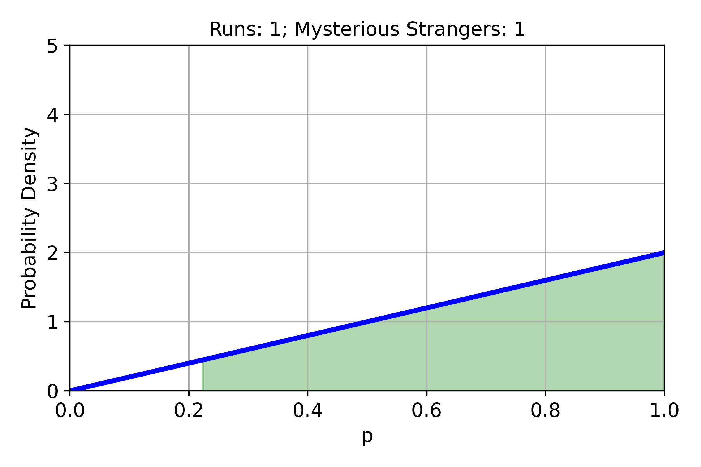
The above plot shows the behavior of the posterior when the amount of data sampled increases. The green area under the graph is the 95% credible region, i.e. there is a 95% chance that the true value for the parameter \(p\) falls inside this region. Now let us consider the last posterior, the one found when using all the 35 sample runs.

After these 35 samples, the most likely chance of getting a Mysterious Stranger when running Avalanchan on normal is 54%. However, even after 35 samples, the 95% confidence region is [38%, 70%], which is a very wide range! It should also be remembered that there is a 5% that the true chance is even outside of this confidence region! Using Bayesian statistics parameters for models of random distributions can be estimated with a confidence region that is easy to interpret. This particular sample size 35 runs highlights how little can be said with certainty when sample sizes are small.

The Python script for the graph can be found here: bayesian_drop_chances.py The creation of the animated graph is based on a blog post by Eli Bendersky.

If you enjoyed this post you can donate a coffee , if you like :)