Bayesian interference of Gaussian parameters

In a previous post Bayesian interference was used to parameter likelyhood of a binomial distribution. The binomial distribution can be used to describe events with discrete probabilities. However, a lot of interesting probabilistic events are continuous. One of the most popular continous probability distributions is the Gaussian distribution. The Gaussian distribution is given as:

\[P(x) = \frac{1}{\sigma\sqrt{2\pi}}\exp\left(-\frac{1}{2}\left(\frac{x-\mu}{\sigma}\right)^2\right)\]

Again let us start from Baye’s theorem:

\[P_\mathrm{posterior}(\theta|D) = \frac{P_\mathrm{likelihood}(D|\theta)P_\mathrm{prior}(\theta)}{P_\mathrm{marginal\ likelihood}(D)}\]

For the Gaussian distribution the data is \(D = \{x_i\}\) and the model parameters are \(\theta = \{\mu,\sigma\}\). Assuming no prior knowledge the prior is approximated to be:

\[P_\mathrm{prior}(\theta) = 1\]

I.e. all parameter values are equally likely when we have no sampels. The likelihood is in general given as:

\[P_\mathrm{likelihood}(D|\theta) = \prod_i P_\mathrm{distribution}(D_i | \theta)\]

Which for the Guassian distribution expands to:

\[P_\mathrm{likelihood}(D|\theta) = \prod_i \frac{1}{\sigma\sqrt{2\pi}}\exp\left(-\frac{1}{2}\left(\frac{D_i - \mu}{\sigma}\right)^2\right)\]

The last needed quantity needed to calculate the posterior is the marginal likelihood:

\[P_\mathrm{marginal likelihood}(D) = \int_\Omega P_\mathrm{likelihood}(D|\theta)P_\mathrm{prior}(\theta)\mathrm{d}\theta\]

Here \(\Omega\) denotes the domain of relevant parameter values. For the Gaussian distribution this turns into a double integral because \(\theta = \{\mu,\sigma\}\):

\[P_\mathrm{marginal\ likelihood}(D) = \int_{\Omega_\sigma}\int_{\Omega_\mu} P_\mathrm{likelihood}(D|\mu, \sigma)P_\mathrm{prior}(\mu,\sigma)\mathrm{d}\mu\mathrm{d}\sigma\]

This integral can be solved analytically, but it is cumbersome, and does not give any insight into how we would do this for an arbitrary distribution. Instead let us solve the integral with numerical integration using Riemann sum:

\[P_\mathrm{marginal\ likelihood}(D) \approx \sum_i^n\sum_j^m P_\mathrm{likelihood}(D|\mu_i,\sigma_j)P_\mathrm{prior}(\mu_i,\sigma_j)(\mu_i-\mu_{i-1})(\sigma_j-\sigma_{j-1})\]

It should be noted that by doing numerical integration the paremeters (\(\mu\) and \(\sigma\)) cannot go to infinity, but we instead have to pick a reasonable upper bound for what they can be. Now everything needed to calculate the posterior is defined. The last step is to define some useful quantities to set a bound on the parameters. The crediable region is defined as:

\[\Omega_{C_R} = \min_\Omega\left|\int_\Omega P_\mathrm{posterior}(\theta|D)\mathrm{d}\theta - C_R\right|\]

Where \(C_R\) is the value of how much credability we want to express our parameters in. The \(\min_\Omega\) is to be read as the smallest continuous \(\Omega\) that will satify the condition. At last we can also determine independt distriutions for the parameters, by integrating out all other parameters. For the Gaussian distribution this will give the two integrals (again to be solved numerically).

\[P_\mathrm{posterior}(\mu| D) = \int_{\Omega_\sigma}P_\mathrm{posterior}(\mu, \sigma | D)\mathrm{d}\sigma\]

and,

\[P_\mathrm{posterior}(\sigma| D) = \int_{\Omega_\mu}P_\mathrm{posterior}(\mu, \sigma | D)\mathrm{d}\mu\]

Let us end with a graphical example. In the following three plots the left and top graphs the distributions where other parameter is integrated out is shown. The green area is the extrema bounds of the crediability region. The central plot shows the credability region of the full posterior, with the credability given by the color. The boundary is the 95% credability. Since we are sampling from a known distribution the true parameter values are marked with a red cross.

First with 5 samples.

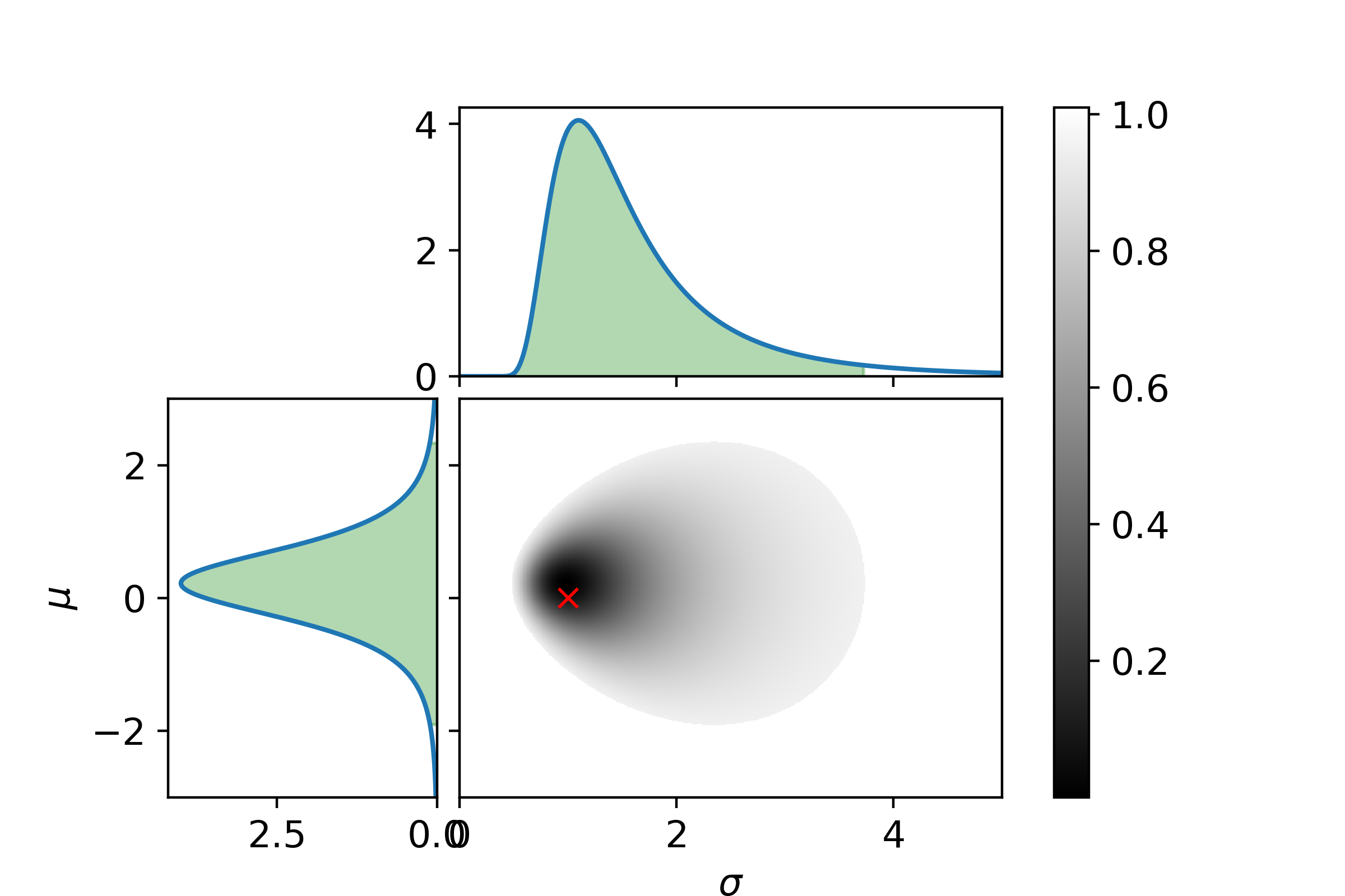
It can be seen with only 5 samples that the parameters are very indetermined. I.e. the 95% crediability region is huge (also remember there is a 5% chance of being outside this region!).

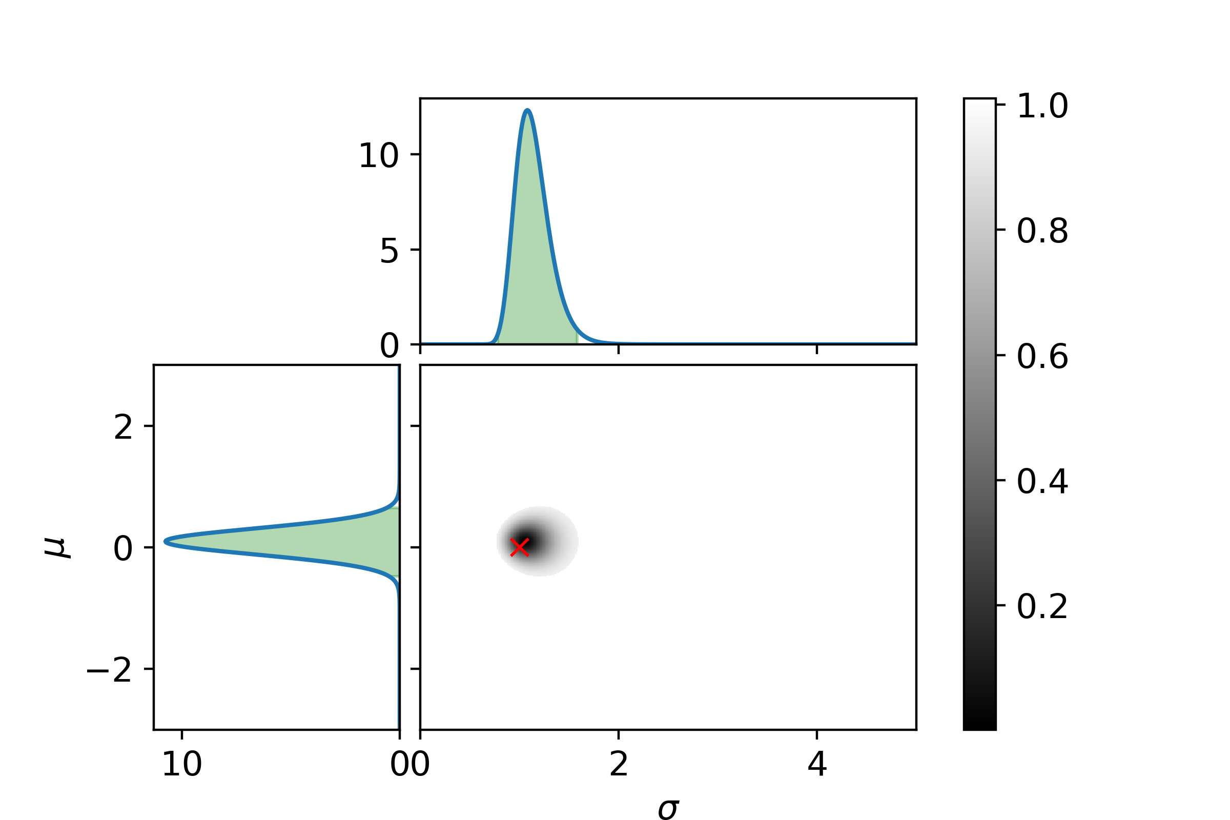
Now with 25 samples.

And at last with 125 samples.

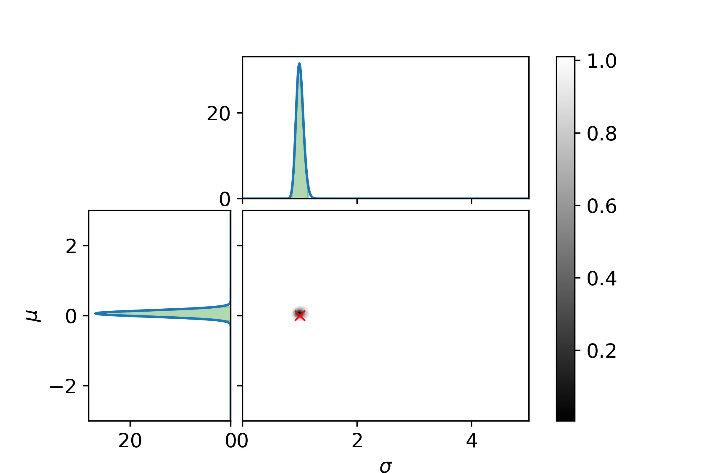
Even with 125 samples the 95% bound is surprisingly large.

The code used to generate the plots can be found here: gaussian_bayesian_example.py

If you enjoyed this post you can donate a coffee , if you like :)