Hellmann-Feynman forces with PySCF
The Hellmann-Feynman theorem states that:
\[\frac{\mathrm{d}E}{\mathrm{d\lambda}} = \left<\psi\left|\frac{\mathrm{d}\hat{H}}{\mathrm{d}\lambda}\right|\psi\right>\]It should be noted that this theorem does not hold for a finite atom-centered basis, and one might want to account for Pulay forces.
For the molecular Hamiltonian:
\[\hat{H} = -\frac{1}{2}\sum_i\nabla_i^2 - \sum_{iK}\frac{Z_K}{r_{iK}} + \sum_{K>L}\frac{Z_KZ_L}{\left|R_{KL}\right|}\]When taking the derivative with respect to the nuclear coordinate it should be clear that:
\[\left<\psi\left|\nabla_K\hat{H}\right|\psi\right> = -\left<\psi\left|\nabla_K\left(\sum_{iK}\frac{Z_K}{r_{iK}}\right)\right|\psi\right> + \nabla_K\left(\sum_{K>L}\frac{Z_KZ_L}{\left|R_{LK}\right|}\right)\]Writing out the two contributions:
\[-\left<\psi\left|\nabla_K\left(\sum_{iK}\frac{Z_K}{r_{iK}}\right)\right|\psi\right> = \left<\psi\left|\left(\sum_{iK}\frac{Z_Kr_{iK}}{r_{iK}^3}\right)\right|\psi\right>\]and,
\[\nabla_K\left(\sum_{K>L}\frac{Z_KZ_L}{\left|R_{LK}\right|}\right) = \left(\sum_{L\neq K}\frac{Z_KZ_LR_{LK}}{\left|R_{LK}\right|^3}\right)\]PySCF uses Libcint for integrals, and it can be seen in the list of available integrals that the derivative of the nuclear attraction operator is unavailable (it is not there). In general the available integrals use the gradient with respect to the electron and not with respect to a nuclei. However, we can realize that:
\[\left<\psi\left|\nabla_e\left(\sum_{iK}\frac{Z_K}{r_{iK}}\right)\right|\psi\right> = \left<\psi\left|\left(\sum_{iK}\frac{Z_Kr_{iK}}{r_{iK}^3}\right)\right|\psi\right> = -\left<\psi\left|\nabla_K\left(\sum_{iK}\frac{Z_{K}}{r_{iK}}\right)\right|\psi\right>\]We can thus write that:
\[-\left<\psi\left|\nabla_K\left(\sum_{iK}\frac{Z_K}{r_{iK}}\right)\right|\psi\right> = \left<\psi\left|\nabla_e\left(\sum_{iK}\frac{Z_K}{r_{iK}}\right)\right|\psi\right>\]Now again we have the problem that this integral with respect to the derivative of the electron coordinate is unavailable, but we can do one more rewrite using partial-integration. Following the derivation done in a previous post, we arrive at the following relation:
\[\left<\psi\left|\nabla_e\left(\sum_{iK}\frac{Z_K}{r_{iK}}\right)\right|\psi\right> = -\left<\nabla_e\psi\left|\sum_{iK}\frac{Z_K}{r_{iK}}\right|\psi\right> -\left<\psi\left|\sum_{iK}\frac{Z_K}{r_{iK}}\right|\nabla_e\psi\right>\]And these two integrals are available as “int1e_iprinv_sph”. The integral can now be computed as:
mol.set_rinv_orig((origin))
grad_nuc_integral = -mol.intor("int1e_iprinv_sph") - mol.intor("int1e_iprinv_sph").transpose(0,2,1)
Obviously, the “mol” object needs to be created as usual with PySCF, and the “origin” will be the center of the atom for which the gradient is calculated. Note that “int1e_iprinv” does not include the nuclear charge, so the result has to be multiplied by \(Z_K\) (this is the case for all atoms, but it is invisible for hydrogen where \(Z_K=1\)).
The integrals are calculated in AO-basis, thus to get the contribution to the nuclear gradient the integrals just need to be contracted with density matrix:
\[\nabla_KE = \sum_{\mu,\nu}D_{\mu,\nu} \left(\nabla_KV_\mathrm{Ne}\right)_{\nu,\mu}\]This contraction can easily be achieved with “np.einsum()”:
rdm1 = mycas.make_rdm1()
nuc_grad_int = mol.atom_charge(atm_idx) * np.einsum('vu,iuv->i', rdm1, grad_nuc_integral)
Now the simple geometry optimizer can be programmed. Using the PySCF molecule object the classical nuclear-nuclear repulsion gradient can be calculated as:
def nuc_grad(mol_obj, nuc_idx):
    coord_nuc = mol_obj.atom_coord(nuc_idx)
    Z_nuc = mol_obj.atom_charge(nuc_idx)
    grad = np.zeros(3)
    for i, (coord, Z) in enumerate(zip(mol_obj.atom_coords(), mol_obj.atom_charges())):
        if i == nuc_idx:
            continue
        grad += Z*Z_nuc*(coord-coord_nuc)/(np.linalg.norm(coord-coord_nuc))**3
    return grad
Calculating the gradients using the previously shown code snippets can be achieved as:
    # Calculate gradients (the forces are the negative gradients)
    gradients = np.zeros((mol.natm, 3))
    for atm_idx in range(mol.natm):
        origin = mol.atom_coord(atm_idx)
        mol.set_rinv_orig((origin))
        grad_nuc_integral = -mol.intor("int1e_iprinv_sph") - mol.intor("int1e_iprinv_sph").transpose(0,2,1)
        rdm1 = mycas.make_rdm1()

        nuc_grad_int = mol.atom_charge(atm_idx) * np.einsum('vu,iuv->i', rdm1, grad_nuc_integral)
        nuc_grad_classical = nuc_grad(mol, atm_idx)

        gradients[atm_idx, :] = nuc_grad_int + nuc_grad_classical
And finally the gradients can be used to move the atoms (the force is the negative gradient, \(F=-\nabla_K E\)). The algorithm used here is the gradient descent. Using gradient descent the coordinates are just updated with the size of the gradient (\(\gamma=1\)):
\[x_{n+1} = x_n - \gamma \nabla E\]In code this can be implemented as:
    # Move atoms and reconstruct molecule
    # Moving using gradient descent
    atom_str = ""
    for atm_idx in range(mol.natm):
        x = (mol.atom_coord(atm_idx)[0] - gradients[atm_idx, 0])/1.8897259886
        y = (mol.atom_coord(atm_idx)[1] - gradients[atm_idx, 1])/1.8897259886
        z = (mol.atom_coord(atm_idx)[2] - gradients[atm_idx, 2])/1.8897259886
        atom_str += f"{mol.atom_symbol(atm_idx)} {x} {y} {z};"
A lot of details in the script have not been described above (only the most important parts). The full script can be found here: hellmann_feynman_pyscf.py
To test if the method works, we can check that the optimizer ends up close to the minimum on the potential energy surface.
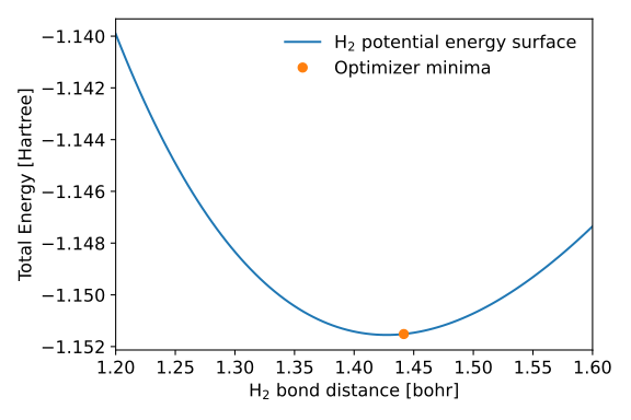
Script to generate the plot can be found here: hellmann_feynman_pyscf_pes_plot.py
As can be seen from the graph, the algorithm using Hellmann-Feynman forces ends up close to the minimum on the potential energy surface of the hydrogen molecule (1.4417 bohr, where the true minimum is at 1.4273 bohr, i.e. about 1% off). The small remaining difference is the Pulay error discussed below.
Pulay forces magnitude
Since we do not have a complete basis, it is known that the Hellmann-Feynman theorem does not hold. We can see how big of an error we are making in the gradient by finding the true gradient using finite differences (with a step of \(\epsilon=10^{-5}\) bohr):
\[\frac{\mathrm{d}f(x)}{\mathrm{d}x} \approx \frac{f(x+\epsilon)-f(x-\epsilon)}{2\epsilon}\]Calculating the gradient like this, and calculating the Hellmann-Feynman gradient, they compare as follows:
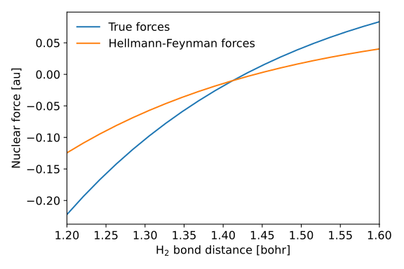
Script to generate the plot can be found here: pulay_forces.py
The difference between the two (the Pulay contribution) is about 0.004-0.007 Hartree/bohr over the plotted range. This is small in absolute terms, but it is of the same size as the gradient close to the minimum. Even more worrying, the Hellmann-Feynman gradient vanishes at a bond distance of 1.4408 bohr, whereas the true minimum is at 1.4273 bohr, so the Hellmann-Feynman forces do not find the exact minimum.
If you enjoyed this post you can donate a coffee , if you like :)